Probabilistic tephra hazard assessment
Tephra describes all fragments of rocks of any size or composition that are injected into the atmosphere during explosive volcanic eruptions. Although tephra is not one of the main causes of casualties in the context of volcanic crisis (tephra are responsible for only 2% of all volcano-related deaths), it can cover wide areas and disrupt a broad range of socio-economic activities. Examples are health problems, collapse of roofs, death of vegetation, blockage of roads and disruption of airports and air traffic. Some hazardous tephra thresholds are shown in the table below. These ranges are wide due to the range of typologies of crops, vegetation, buildings that can be impacted, as well as external factors (e.g. time of the year for crops). Refer to the references provided in the previous lesson for more information on how to quantify physical vulnerability to tephra fallout.
| Element | Threshold (\(kg/m^{2}\)) |
|---|---|
| Airport closure | 1 |
| Perturbation of the road network | 1-100 |
| Impact on crops | 5-150 |
| Impact on vegetation | 5-1500 |
| Roof collapse | 100-300 |
Objectives
The aim of this exercise is to compile a probabilistic hazard assessment for tephra accumulation for a future eruption at La Palma. Probabilistic modeling will be performed using the model Tephra21 and the Matlab toolbox TephraProb2.
In this exercise, you will use the user-friendly Matlab toolbox called TephraProb to:
- Analyse the eruptive record and perform some basic frequency analyses.
- Analyse the wind patterns in a region and put this in the perspective of the hazard assessment.
Running the full workflow for probabilistic hazard assessment in the computer lab is complicated by technical issues (e.g., computation time, compilation of source libraries). Therefore, we have already ran the scenario for you. You will nevertheless:
- Learn how to interpret the sampling of ESP.
- Analyse the hazard outputs.
TephraProb
For more information about TephraProb, you can refer to the:
- Video tutorial.
- Updates on the code's website.
Getting started
Setup TephraProb
The VolcanicRisk2023.zip located on Moodle contains folder named TephraProb, which we will use throughout the exercise.
Alternative link
- Start
Matlab. If your computer has several versions, use the latest one. - Left of the address bar at the top of the main
Matlabwindow, click on the iconBrowse for Folderand navigate to the location ofTephraProb(i.e. the location of the filetephraProb.m). - In the Matlab command line, type
TephraProband press enter to startTephraProb.
Use your user disk!
If you are using the PC of the computer lab, make sure your files are saved on your personal drive! This is typically the H:\ drive. Otherwise, your files will be deleted every time you logout!
Hazard assessment
This exercise is structured in 3 parts:
- Analysing wind patterns at la Palma using the EMCWF ERA-5 database.
- Defining an eruption scenario and associated ESP.
- Analysing the hazard output.
VEI and plume height
The VEI scale suggests very approximative indications of plume height for each VEI class. For instance, it suggests heights of 1-5 km for VEI 2 and 3-15 km for VEI 3 eruptions. However, the VEI scale does not include any information about intensity of the eruption (→ duration over which the VEI volume was erupted).
The volume associated with the 2021 VEI 3 eruption was erupted over the course of a few months, but plume heights were in the 1-5 km range rather than the 3-15 km range. Therefore, let's consider here the following plume heights:
- VEI 2: 1-5 km.
- VEI 3 - low intensity: 1-5 km (→ long-lasting eruption lasting for days/weeks).
- VEI 3 - high intensity: 3-15 km (→ intense eruption lasting for hours).
Wind data analysis
In order to take into account the aleatoric variability of atmospheric conditions in the hazard assessment, a large population of wind profiles is required from which a different wind profile is randomly sampled at each model run. The atmospheric database used here is the EMCWF ERA-5 database.
Downloading atmospheric data takes time - we have therefore already prepared the dataset for you. The dataset contains 5 years of wind for the period 2017-2021, providing 4 wind profiles per day at a resolution of 0.25 degrees (e.g., ~28 km at the equator) above La Palma.
Wind population
For the purpose of the exercise, we are using 5 years of wind data, which facilitates file transfer and speed up analyses. Keep in mind that we usually use larger populations for real applications (typically more than 10 years depending on the variability in a given region).
Analysing wind patterns
You can now display wind profiles. Keep your eyes opened for seasonal trends in both wind direction and speed.
- On the main
TephraProbwindow, clickInput>Wind>Analyze wind - Select the
wind.matfile located inWIND/CumbreVieja_1721/ - A new panel opens, on which you can explore wind profiles either using
wind profilesorwind roses.
Wind profiles
Wind profiles show wind velocity and wind direction as a function of altitude. Wind profiles can be plotted either separately (e.g., one wind profile per year or per month) or averaged (e.g., mean ± standard deviation).
Wind rose
Wind roses show the probability (concentric circles) of the wind blowing in each direction [0 - 360 degrees]. Colours indicate wind velocity. Wind roses are plotted for a given elevation, so explore a few.
Question 1: Wind conditions
- Visualize these wind patterns in the context of a hazard assessment. What is the main wind direction?
- Can you observe a seasonality in wind patterns?
Eruption scenario
Let's try and forget what we know about the 2021 eruption and put ourselves in this reasoning framework:
- We need to assess the hazard associated with tephra accumulation for a future eruption along the Cumbre Vieja rift.
- From the historical record, most eruptions are VEI 2. However, since what we observed in the field deposits seems larger than VEI 2 eruptions, we decide to focus on a VEI 3 eruption.
- However, the deposits we observed do not look like short-lasting, subplinian VEI 3 eruptions. We suspect that these eruptions were less intense and longer-lastin. We therefore model an eruption lasting between 3 days to one week with plume heights varying between 1-5 km.
- We have no information regarding the grain-size distribution of the observed deposits, and therefore decide to use an analogue eruption to inform us. We chose the 2002 eruption of Etna volcano.
Grain size distribution
For clarity, we haven't touched yet on the concept of grain-size distribution or GSD. This is an important ESP for tephra dispersal as it controls how fine (or coarse) the tephra generated at fragmentation level will be, and therefore will control how far particles will go.
Grain size is expressed in \(\Phi\) units, which is calculated as \(-log_2(d)\), where \(d\) is the particle diameter in \(mm\). In \(\Phi\) units:
- A 1 mm-particle has \(\Phi=0\).
- Particles coarser than 1 mm have negative \(\Phi\) values.
- Particles finer than 1 mm have positive \(\Phi\) values.
In Tephra2 the GSD of the model deposit is considered to be a Gaussian distribution centered on \(Md_\Phi\) (i.e., mean) and varying by \(\sigma_\Phi\) (i.e., standard deviation).
See what we just did? We just defined an eruption scenario! The table below summarises the ESP for our low-intensity VEI 3 eruption.
| ESP | Value | Description |
|---|---|---|
| VEI | 3 | Similar to the 2021 eruption |
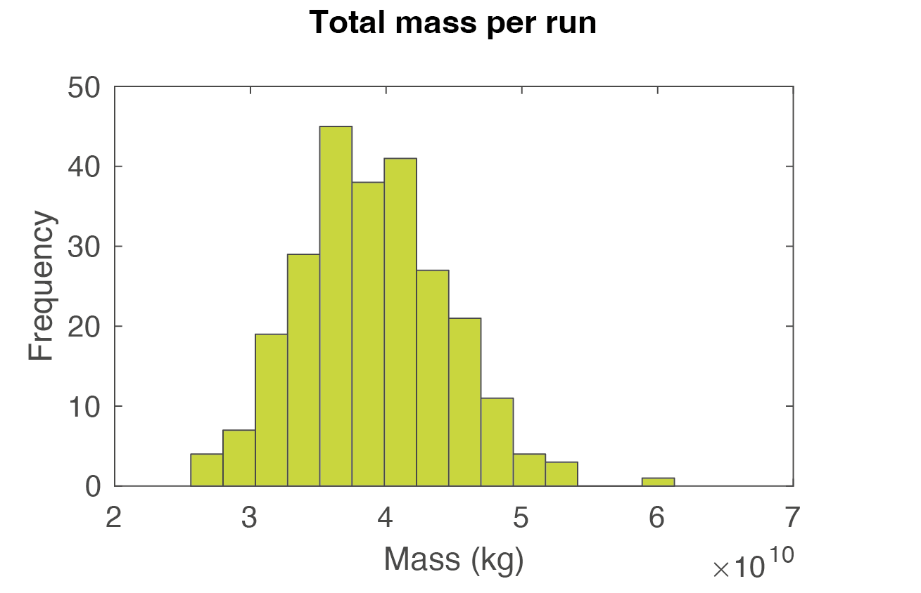
| Mass | 10\(^{10}\)–10\(^{11}\) kg | Using the volume ranges of a VEI 3 eruption and conversion to mass using a bulk deposit density of 1000 \(kg/m^{3}\) |
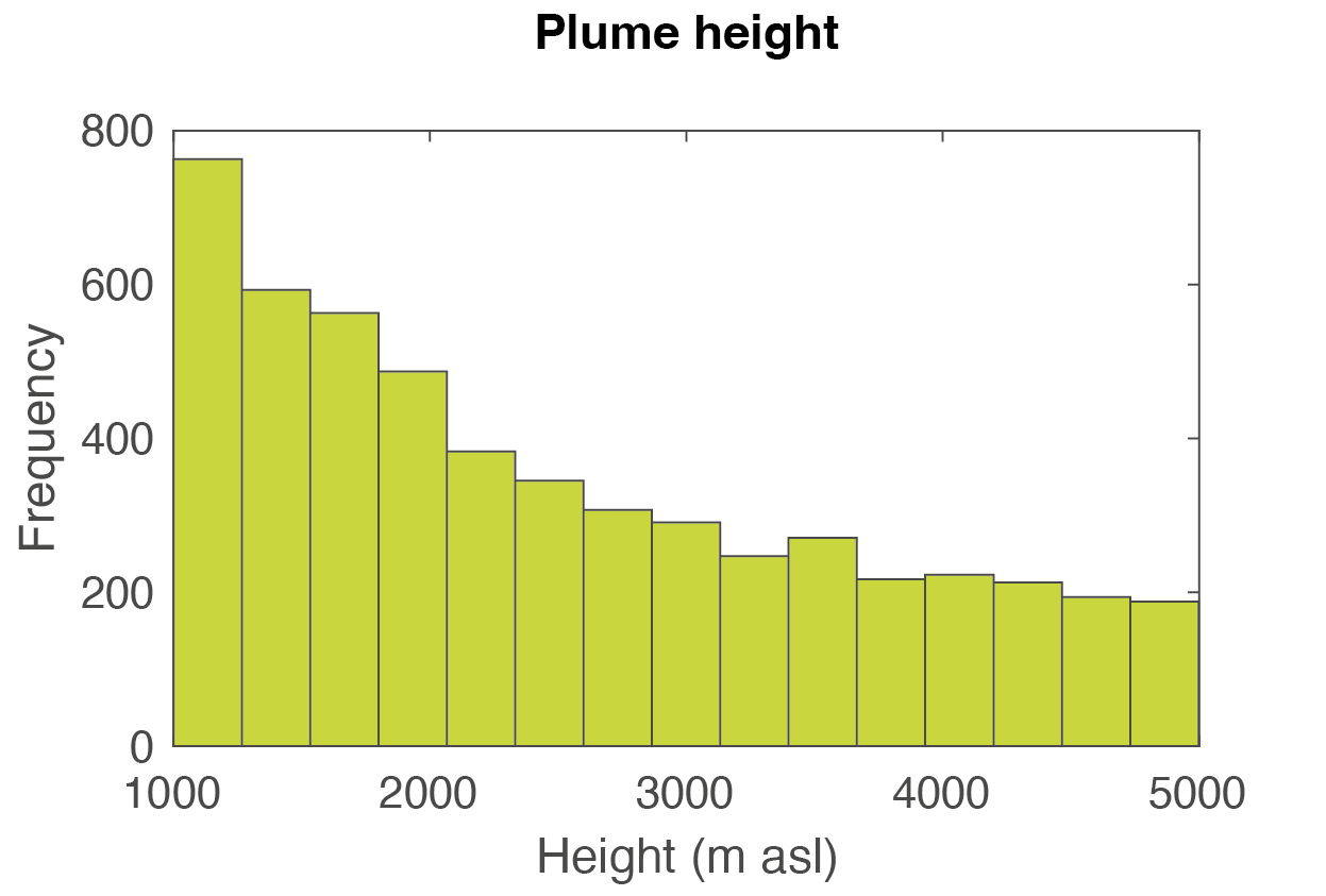
| Height | 1-5 km | Low intensity VEI 3 eruption occurring over a few days |
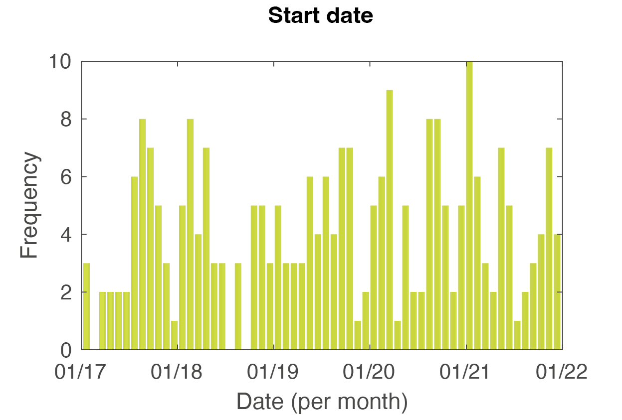
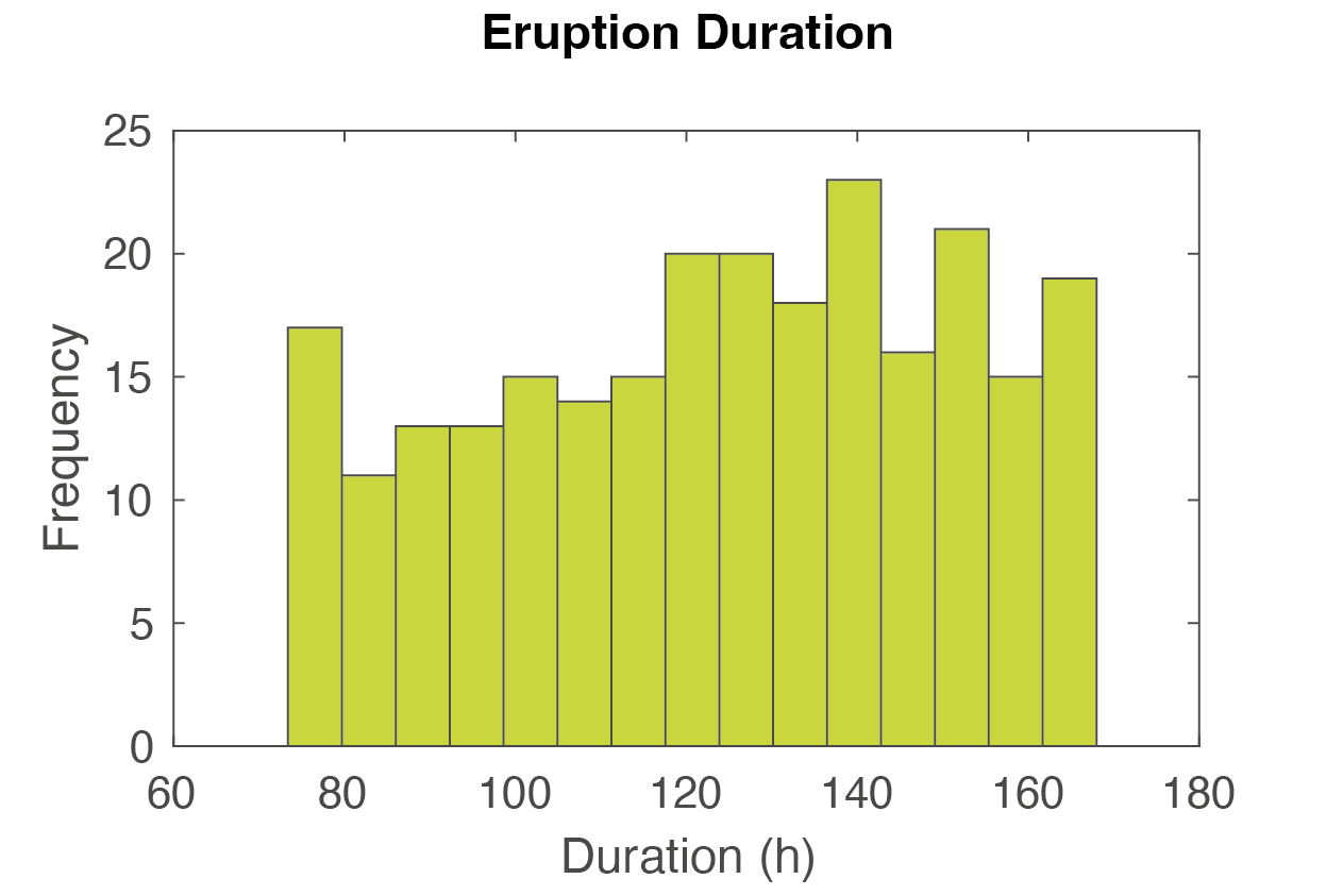
| Duration | 3-7 days | Paroxysmal phase of a longer eruptive sequence |
| Md\(_\Phi\) | 0-1 \(\Phi\) | Center of the grain-size distribution, based on Etna 2002 |
| \(\sigma_\Phi\) | 1-2 \(\Phi\) | Spread of the grain-size distribution, based on Etna 2002 |
ESP sampling
Now that we have defined the ranges of ESP, TephraProb applies the algorithm below to sample \(n\) sets of ESP. For the sake of the exercise, \(n\) is here set to 250 runs. The figures below summarise the sampling of the ESP.
flowchart TD

subgraph sg0 ["Eruption scenario"]

A1["HEIGHT [min, max]"]
C1["DATE [min, max]"]
B1["DURATION [min, max]"]
D1["MASS [min, max]"]

end

subgraph sg1 ["For each run"]

    subgraph sg2 [" "]
        A2["Sample Height"]
        C2["Sample Date"]
        B2["Sample Duration"]
    end


C2 --> C3["Get wind velocity"]
C3 --> E["Calculate MER"]
A2 --> E
E --> F["Calculate simulation Mass"]
B2 --> F

F --> G["Is Mass within MASS [min, max]"]
D1 --> G

end

A1 --> A2
C1 --> C2
B1 --> B2

G --> H1[Yes]
G --> H2[No]

H1 --> I1["Run is valid, move to next one"]
H2 --> I2["Run is not valid, restart"]
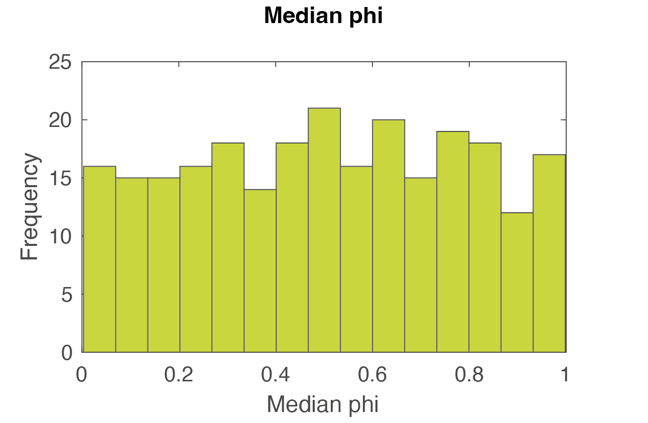
Question 2: ESP
Analyse the distributions of sampled ESP. For each ESP, discuss:
- From what distribution have each ESP been sampled from? (Hint: there are three types of distributions used here: logarithmic, normal and uniform).
- What prior knowledge do these three distributions reflect?
Hazard output
Question 3: Probability calculation
-
The previous module has introduced how to compute exceedance probability for tephra accumulation. Based on the 10 simulations below for pixel \(x,y\), what are the probabilities of this pixel to suffer tephra accumulations exceeding:
- 50 \(kg/m^2\)?
- 100 \(kg/m^2\)?
- 150 \(kg/m^2\)?
| Simulation | Tephra accumulation (\(kg/m^2\)) | Simulation | Tephra accumulation (\(kg/m^2\)) |
|---|---|---|---|
| 1 | 115 | 6 | 156 |
| 2 | 80 | 7 | 102 |
| 3 | 151 | 8 | 104 |
| 4 | 65 | 9 | 85 |
| 5 | 112 | 10 | 123 |
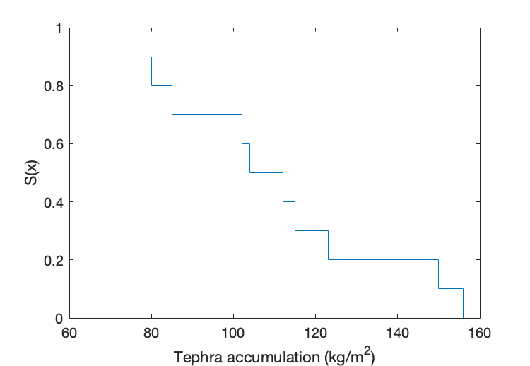
-
Similarly, we also learned how to estimate a typical accumulation associated with a given probability of occurrence. The figure below shows the survivor function for the data in the table above. Estimate the approximative load associated with probability values of:
- 30%
- 70%
Load runs
One single vent was assigned to each of you. For the rest of the exercise, make sure you refer only this one.
Let's now load your assigned scenario, where runName goes from vent1 to vent5:
- On the main
TephraProbwindow, clickFile>Open - Select the
.matfile located inRUNS/runName/1/
Probability maps
Probability maps fix a critical value of tephra accumulation (\(kg/m^2\)) to allow the contouring of the spatial probability of exceeding this critical threshold. These maps are useful to see the dispersion of probabilities across an area, but only for one given tephra accumulation threshold at the time.
Let's plot probability maps:
- Make sure the scenario for the vent that was attributed to you is loaded (
File > Load). - From the main
TephraProbwindow, clickDisplay > Probability Maps. - A new window opens, from which you can select pre-defined accumulation threshold (you can select multiple using the Cmd (Mac) or the Ctrl (Windows) keyboard buttons). Do not open all maps! Select only the 1 10, 100 \(kg/m^2\).
- Click
Ok-Google Earth should now open.
Troubleshooting Google Earth
If Google Earth is in French:
Google Earthis in French by default. To change the language, go toOutils/Options/General/Parametres de langueand choose your language.
If Google Earth does not open:
- From the main
TephraProbwindow, selectFile > Preferencesand make sure theShow Google Earthoption is selected.
Probability maps
No question to answer here, but take a moment to think about:
- In which direction (i.e., downwind cardinal reference) is the hazard associated with tephra fallout most likely to occur?
- At each point of the map, can you express exactly the information that is presented?
Probabilistic isomass maps
Probabilistic isomass maps fix a probability threshold to represent a typical tephra accumulation given a probability of occurrence of the hazardous phenomenon. The choice of the probability threshold, which can be regarded as an acceptable level of hazard, is a critical aspect that is the resort of decision-makers. Scientists should therefore communicate results from probabilistic isomass maps with care.
To plot probabilistic isomass maps:
- From the main
TephraProbwindow, clickDisplay > Isomass Maps. - A new window opens, from which you can select pre-defined probability thresholds. Choose the 25% and 75%.
- Click
Ok-Google Earth should now open.
Probabilistic isomass maps
Again, no question to answer, but reflect on:
- What are these maps showing?
- How do they differ from probability maps?
Hazard curves
Let's now look at hazard curves. For each vent, hazard curves for three points have been processed. To visualise them:
- From the main
TephraProbwindow, chooseInput > Points. - From the new window, chose
File > Loadand select theGRID/LaPalma_ventX/LaPalma_ventX.pointsfile. - The points appear, click
Plotto visualise them.
Relevant points to each vent regarding the hazard to roof collapse are presented in the table below. To plot hazard curves:
- From the main
TephraProbwindow, clickDisplay > Hazard curves - Choose the point for your own vent as named in the table below.
| Location | Longitude | Latitude |
|---|---|---|
| El Paso, houses | -17.85992 | 28.65247 |
| Location | Longitude | Latitude |
|---|---|---|
| San Nicola, houses | -17.88052 | 28.60222 |
| Location | Longitude | Latitude |
|---|---|---|
| Jedey, houses | -17.87995 | 28.58373 |
| Location | Longitude | Latitude |
|---|---|---|
| El Pueblo, houses | -17.77892 | 28.60605 |
| Location | Longitude | Latitude |
|---|---|---|
| Los Canarios, houses | -17.84446 | 28.49251 |
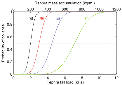
Figure 1 represents fragility curves for various European roofs (Spence et al., 20055), and estimate a median probability of roof collapse as a function of tephra accumulation. Use these curves to answer the following questions.
Question 4: Hazard curves
For the point attributed to your vent, use the model of Spence et al. (2005)5 to estimate a probability of occurrence of roof collapse. To convert a mass per unit area (\(M\), \(kg/m^2\)) to a load (\(L\), \(kPa\)), use:
- Assuming that the considered buildings are of a MS fragility class, what are the probabilities of roof collapse for associated with mass loads for 25% and 75% probability of occurrence?
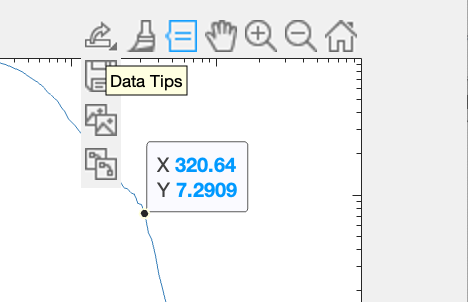
Accessing hazard curves with data tips
On the hazard curve figure, you can activate the Data Tips tool. This allows you to click on the curve and directly get the underlying data. It is hard to get exact probabilities, so anything within a ± 5% range is ok.
Estimating probability of roof collapse
Once you have estimated the load, you can read the corresponding probability of roof collapse from Figure 1. If you feel adventurous, you can also compute it directly from the Matlab command line (where \(L\) is the load):
Note that the MS class according to Spence et al. (2005)5 is characterised by:
1. A normal cumulative density function
2. A mean value of 4.5 kPa
3. A standard deviation of 20%
Refer to the original paper for more information.
Food for thoughts
Well done - you have successfully completed a scenario-based probabilistic hazard assessment for tephra accumulation! Keep in mind that:
- The scenario-based part implies that this hazard is contitional to the occurrence of the eruption scenario. This contrasts with a fully probabilistic volcanic hazard assessment, where the spatio-temporal probability of occurrence of given volcanic phenomena also need to be accounted for.
- Having pretty maps is great... but knowing how to communicate the hazard output and the associated assumptions and uncertainties is often equally important. Keep that in mind for the rest of the exercises, both in the lab and in the field.
Getting the hazard data
As displayed in Matlab, you can save the maps displayed within TephraProb by simply typing saveAllMaps('png'), which will save all opened maps to TephraProb/MAPS. The raw output data for both probability and isomass maps are saved as ascii raster file with a UTM 28 N projection. Probability (PROB) and isomass (IM) data are located in:
These are useful for use in external softwares (e.g., QGIS). Similarly, kml files are stored in the KML folder of your run.
Hazard curves must be saved from within Matlab.
Summary
This module provided a practical application of the concepts introduced in the previous module, using La Palma as a case study and producing a scenario-based hazard assessment for tephra accumulation using TephraProb.
References
-
Bonadonna, C., Connor, C.B., Houghton, B.F., Connor, L., Byrne, M., Laing, A., Hincks, T.K., 2005. Probabilistic modeling of tephra dispersal: Hazard assessment of a multiphase rhyolitic eruption at Tarawera, New Zealand. J. Geophys. Res 110, 2156–2202. ↩
-
Biass, S., Bonadonna, C., Connor, L., Connor, C., 2016. TephraProb: a Matlab package for probabilistic hazard assessments of tephra fallout. Journal of Applied Volcanology 5, 1–16. ↩
-
Simkin, T., Siebert, L., Simkin, T., Kimberly, P., 2010. Volcanoes of the World. University of California Press, Tucson, AZ. ↩
-
Jenkins, S.F., Wilson, T.M., Magill, C., Miller, V., Stewart, C., Blong, R., Marzocchi, W., Boulton, M., Bonadonna, C., Costa, A., 2015. Volcanic ash fall hazard and risk, in: Loughlin, S., Sparks, S., Brown, S., Jenkins, S., Vye-Brown, C. (Eds.), Global Volcanic Hazards and Risk. Cambridge University Press, pp. 173–222. ↩
-
Spence, R.J.S., Kelman, I., Baxter, P.J., Zuccaro, G., Petrazzuoli, S., 2005. Residential building and occupant vulnerability to tephra fall. Natural Hazards and Earth System Sciences 5, 477–494. ↩↩↩